In this project, I tried to build a Automatic Speech Recognition system in my mother tongue, Hindi. I undertook this project to explore the two famous toolkits for building ASR Systems: HTK and Kaldi. I can proudly say that I learned a lot in this project and can now easily build any system using the two toolkits. Here I didnt merely understand how to write code to use the toolkits but also understood in depth the underlying processes/mathematics taking place at each step. I would like to thank Prof Samudravijaya K (CLST , IIT Guwahati) and Sreeram Ganji bhaiya (PhD , IIT Guwhati) for their constant support and help in clarifying my numerous doubts along the course of the project.
In total I implemented 4 systems:
1)Monophone-HMM system built using HTK toolkit
2)Monophone-HMM system built using Kaldi
3)Triphone-HMM system built using Kaldi
4)DNN-HMM system built using Kaldi
The code for the entire project is available on my GitHub page : https://github.com/KunalDhawan/ASR-System-for-Hindi-Language
I would try to explain each and every step as taken by me for building the ASR system in this documentation. Thus starting from the first step, that is Data Collection
Data Collection
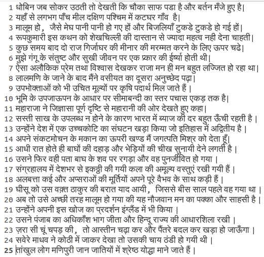
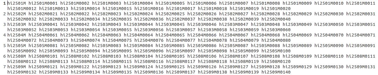
The first step here was to compile 150 grammatically rich sentences in Hindi having maximum possible unique words and trying to capture distinct situations . Obviously the more the number of unique sentences (and words), the better would be the performance of the recognition system
Shown below are few of the sentences that were chosen-
In total I implemented 4 systems:
1)Monophone-HMM system built using HTK toolkit
2)Monophone-HMM system built using Kaldi
3)Triphone-HMM system built using Kaldi
4)DNN-HMM system built using Kaldi
The code for the entire project is available on my GitHub page : https://github.com/KunalDhawan/ASR-System-for-Hindi-Language
I would try to explain each and every step as taken by me for building the ASR system in this documentation. Thus starting from the first step, that is Data Collection
Data Collection
The first step here was to compile 150 grammatically rich sentences in Hindi having maximum possible unique words and trying to capture distinct situations . Obviously the more the number of unique sentences (and words), the better would be the performance of the recognition system
Shown below are few of the sentences that were chosen-
The next step was Transliteration of the sentences from devanagari script to ILSL12 convention (which is used by Indian speech R&D community). This was done by first converting Indian-language text from UTF-8 Unicode Devanagari to ISCII format and then from ISCII to ILSL12 convention. For the first two sentences were finally converted to-

Parallelly , I created the phone level decomposition for each of the sentences , following the ILSL 12 convention. The transliteration produced above also had to be rectified at some places depending upon the actual phone used while pronouncing a word in a sentence, which was sometimes incorrectly detected by the hard coded transliteration code used above , which just converted on the basis of occurrence of the symbol for the phone, but not on the basis of the sound as required. This is because in Hindi and many other languages , the same symbol can correspond to different sounds depending on the phones surrounding it. This effect is known as co-articulation. On such example is the bindu (also known as nukta) in Hindi, which will sound differently based on the place of articulation of the phone on it's right. The following document presents the ILSL symbol for the different sounds in Hindi :
One easier way to correct for the inaccurate transliteration is let the sentence level transcription remain the same as above and account for the correct phone corresponding to the word while creating the lexicon. In the lexicon, we basically mention the correct sequence of phones in all the possible words as present in our training data. This is because when we build the monophone/ triphone model, we would like to model each phone as a state. Thus the toolkit internally would first look as the transliteration corresponding to each spoken sentence and then for each word, look at the phonetic decomposition correspondingly from the lexicon , thus finally form a file containing the phone level decomposition of each sentence, which it will use for training the model. The first few entries of the lexicon for my data is as follows:-
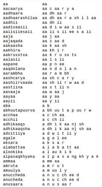
One should ensure that all the words present in the transliteration file should be present here. A good way of preparing the first column will be to sort the words words from transliteration file in alphabetical order and then take the unique words from it using simple bash commands
Next step was to record the data. I had 7 speakers(including myself) , who have Hindi as their mother tongue and use it for their daily communication, speak out the 150 sentences I had collect. Multiple speakers were required to train a speaker- independent model, ie the model should ideally not depend on the speaker who is speaking , which would have been the case if we had used just 1 speaker data to train the model.
So finally I have 150*7= 1050 utterances. Out of that I used 20 different mutually exclusive sentences from each speaker for testing (ie 7*20=140 test sentences) and the remaining 910 sentences were used to train the model.
You can listen to the wav files via the following link - drive.google.com/open?id=1YZb7ZOUKspPHwBX12wJf-7_wm2i_JwO3
Next for Building the model, the steps differ for HTK and Kaldi. So Next I branch to two section- 1st for HTK and 2nd for Kaldi. Both of them work on the same data as prepared above.
Building the Monophone-HMM ASR system using HTK
I will try to explain the working alongside the method to run the code I have put up on GitHub. The link to the code is github.com/KunalDhawan/ASR-System-for-Hindi-Language/tree/master/HTK
First Step would be to provide the scripts present in the folder scripts_sh_pl_py read write permissions. This is done on linux by going to the above directory and running the command
>chmod a+rx *.sh *.pl *.py
Next we come back to the parent directory (by cd ..) and the run the command:
>scripts_sh_pl_py/master.sh HCOPY
This runs the HCOPY script present in the folder (the master.sh file correctly initializes the environment variables and also contains the code for writing into the log directory after every big command)
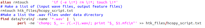
This script first creates a corresponding .mfc file for each audio sample present in the data directory using the following c shell (and perl) code and writes them in the file hcopy_script.txt under the htk_files folder. This file name will be used to store the extracted MFCC features for each audio file) -
Next step was to record the data. I had 7 speakers(including myself) , who have Hindi as their mother tongue and use it for their daily communication, speak out the 150 sentences I had collect. Multiple speakers were required to train a speaker- independent model, ie the model should ideally not depend on the speaker who is speaking , which would have been the case if we had used just 1 speaker data to train the model.
So finally I have 150*7= 1050 utterances. Out of that I used 20 different mutually exclusive sentences from each speaker for testing (ie 7*20=140 test sentences) and the remaining 910 sentences were used to train the model.
You can listen to the wav files via the following link - drive.google.com/open?id=1YZb7ZOUKspPHwBX12wJf-7_wm2i_JwO3
Next for Building the model, the steps differ for HTK and Kaldi. So Next I branch to two section- 1st for HTK and 2nd for Kaldi. Both of them work on the same data as prepared above.
Building the Monophone-HMM ASR system using HTK
I will try to explain the working alongside the method to run the code I have put up on GitHub. The link to the code is github.com/KunalDhawan/ASR-System-for-Hindi-Language/tree/master/HTK
First Step would be to provide the scripts present in the folder scripts_sh_pl_py read write permissions. This is done on linux by going to the above directory and running the command
>chmod a+rx *.sh *.pl *.py
Next we come back to the parent directory (by cd ..) and the run the command:
>scripts_sh_pl_py/master.sh HCOPY
This runs the HCOPY script present in the folder (the master.sh file correctly initializes the environment variables and also contains the code for writing into the log directory after every big command)
This script first creates a corresponding .mfc file for each audio sample present in the data directory using the following c shell (and perl) code and writes them in the file hcopy_script.txt under the htk_files folder. This file name will be used to store the extracted MFCC features for each audio file) -
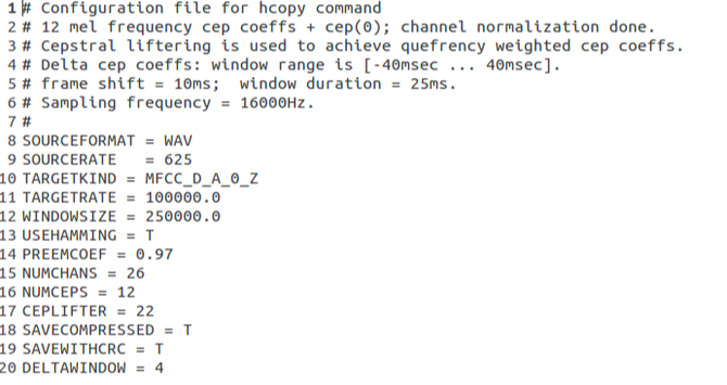
Next this invokes the inbuilt function HCopy of the HTK toolkit which is used for feature extraction from the wav data . We extract 12 MFCC coefficient and the 0th cepstral coefficient. The parameters for this feature extraction process are written in a config file and passed on to HCopy as one of the input arguments. The snapshot of the config file for the HCopy command is attached bellow:
Next we run the command-
>scripts_sh_pl_py/master.sh LEXICON
This call the scripts writeTranscription.sh and create_lm.sh from within the master.sh script which sets the appropriate environment variables.
This script generates in the lm directory files containing-
- Transcriptions
- Master Label Files at phone level and word level
- Bigram grammar files
- lists of symbols (monophones0 and monophones1)
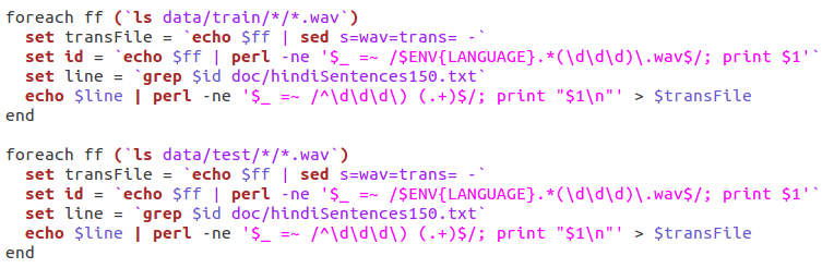
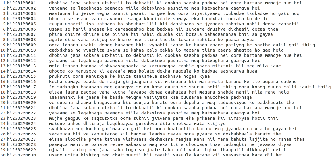
The script writeTranscription.sh takes the transcription corresponding to the sentence id as present in file hindiSentences150.txt that was prepared by me earlier and stores them in .trans format with each .wav file present in my data directory. This is done via the following script-
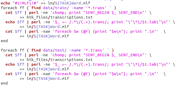
Next we call the script create_lm.sh which is used to generate a file containing transcriptions and Master Label Files at phone level and word level, Bigram grammar file and lists of symbols (monophones0 and monophones1). This done by using the inbuilt HTK commands.
The commands LNewMap, LGPrep, LGCopy, LBuild and HBuild are used to build the bigram grammar.
Next we manually create the word level MLF (Master Label File) according to the HTK format. This is done by using the transcription files for each .wav sample(test and train) created earlier and manipulating it as follows:
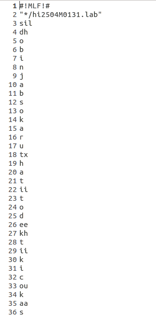
Once the word level MLF has been created, phone level MLFs can be generated using the label editor HLEd(inbuilt HTK command).
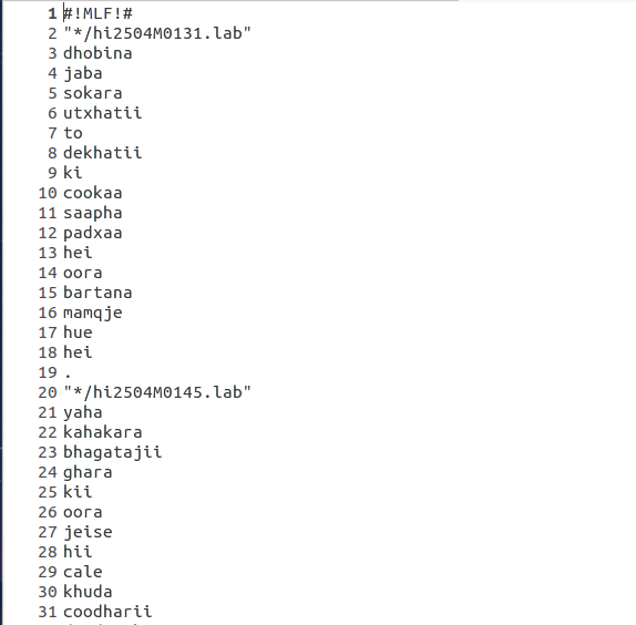
Presented bellow is a snapshot of the word level MLF and phone level MLF files.
Presented bellow is a snapshot of the word level MLF and phone level MLF files.
Next , using a simple script , we convert the phone level MLF file to symbol list , which is basically a collection of all unique phones in alphabetical order. Let us call this file monophones0 (as suggested in the HTK Tutorial). Then we create another file monophones1 in which we add the short pause symbol 'sp'.
The next command is
>scripts_sh_pl_py/master.sh HCOMPV
This call the scripts hcompv.sh from within the master.sh script which sets the appropriate environment variables. This script performs the step 6 of chapter 3 of the HTK Tutorial. First we create directories to hold the various versions of the HMM models( as per my code , we will have 10 models). Here we use all training files to compute global means & variances of features and set the means & variances of all state pdfs of the prototype HMM to the global ones. This is done via the inbuilt command HCompV. Here we set the config file such that delta and acceleration coefficients are also computed and appended to the static MFCC coefficients computed earlier. This process is known as flat-start. Basically we initailize the PDF of each of the phoneme model equal to the mean and covariance of the entire training data .
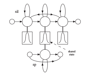
Here because we are building a monophone system, thus each phone emission is modelled by a gaussian mixture model and the transition probabilities between the phones is modelled by an HMM. Thus each phone is modelled by a 5 state HMM in which the first and last states are non-emitting and the probability of the rest 3 states emitting are modelled by gaussians. An excellent resource for understanding HMMs better is this awesome paper/tutorial by prof Rabiner - www.ece.ucsb.edu/Faculty/Rabiner/ece259/Reprints/tutorial%20on%20hmm%20and%20applications.pdf
Next we re-estimate the parameters for the HMMs . This is done by the command
>scripts_sh_pl_py/master.sh HEREST
This command calls the script herest.sh which re-estimate parameters of HMM models using embedded re-estimation (also called Baum-Welch re-estimation equations). This step is performed by the the inbuilt HTK command HERest. It would be difficult to explain the embedded re-estimation algo here, for that an excellent resource is online video lectures by prof Samudravijaya www.youtube.com/channel/UCHk6uq1Cr9J3k5KNmIsYUNw.
Trying a short explanation- A HMM can be uniquely specified using the parameters 1)state transition probability distribution A, 2)The observation symbol probability distribution B and 3)The initial state distribution pi. The iterative estimation of these parameters is given by the formula(source- page 9 of Rabiner sir's paper as mentioned above)
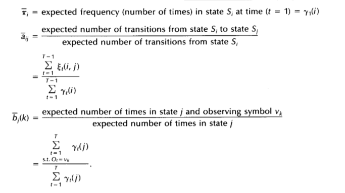
I perform this re-estimation 3 times to have a good fit to the data .
Next we go on to fix the silence model. The thing wrong with out model right now is that mostly while speaking , we introduce a short pause between adjacent words. This pause is slightly smaller than silence and may/may not occur. But right now we havent trained a model for short pause, we have just trained models for all phones and for silence. Thus , to fix our system , we introduce a short pause HMM between all adjacent HMM that we had after the above step. The short pause model is obtained by taking the trained silence model, keeping only the first and last non-emitting stages and only the middle emitting stage, and adding a transition from the first to the last stage . so that the sp model need not necessarily emit each time . This can be depicted pictorially as-
Next we go on to fix the silence model. The thing wrong with out model right now is that mostly while speaking , we introduce a short pause between adjacent words. This pause is slightly smaller than silence and may/may not occur. But right now we havent trained a model for short pause, we have just trained models for all phones and for silence. Thus , to fix our system , we introduce a short pause HMM between all adjacent HMM that we had after the above step. The short pause model is obtained by taking the trained silence model, keeping only the first and last non-emitting stages and only the middle emitting stage, and adding a transition from the first to the last stage . so that the sp model need not necessarily emit each time . This can be depicted pictorially as-
Now after fixing the silence model, we call the re-estimation script 2 times again so that it adapts the parameters to the changes we have made.
Right now, the dictionary may contain multiple pronunciations for some words, particularly function words. The phone models created so far can be used to realign the training data and create new transcriptions. This can be done with a single invocation of the HTK recognition tool HVite. To do this , we execute the statement:
>scripts_sh_pl_py/master.sh ALIGN
This call the scripts hviteAlign.sh from within the master.sh script which sets the appropriate environment variables. hviteAlign.sh realigns the training data using HMMs created so far and it creates new transcriptions (with best pronunciation [out of many alternatives] for each recognised word) for aligned/training data.
After this herest.sh is again called to perform 2 re-estimation cycles
Next , we evaluate the performance of our system on the not-seen-before test data. For this we execute
>scripts_sh_pl_py/master.sh HVITE_MONO
This evaluates the performance on test data using the inbuilt function HVite and then show the results using the function HResults .
The final output is -
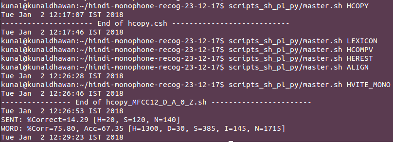
Thus I successfully built an ASR system for hindi language, which gives good result given the fact that this is a very simple system. We can even extend this to using the trained models for recognition of live Audio, ie speech samples taken from microphone on laptop. This can be done via the script LiveDemo in the folder.
With this I move on to Kaldi. One advantage I found of using Kaldi is that the number of gaussian for each model is not same unlike in HTK. Here the script automatically finds the best number gaussian for each model independently and just ensures that those are less than the upper limit we specify ( I will explain this is detail with the code snippets later). Thus Kaldi gives relatively better performance than HTK given the same data and architecture.
With this I move on to Kaldi. One advantage I found of using Kaldi is that the number of gaussian for each model is not same unlike in HTK. Here the script automatically finds the best number gaussian for each model independently and just ensures that those are less than the upper limit we specify ( I will explain this is detail with the code snippets later). Thus Kaldi gives relatively better performance than HTK given the same data and architecture.
Kaldi Implementation
1) Monophone HMM System
First step here is to run the script file path.sh that has been created to load all binaries required for the implementation
Here , we store the .wav files in the folder wav. Here too like HTK I have 150*7= 1050 utterances. Out of that I used 20 different mutually exclusive sentences from each speaker for testing (ie 7*20=140 test sentences) and the remaining 910 sentences were used to train the model.
You can listen to the wav files via the following link - drive.google.com/open?id=1YZb7ZOUKspPHwBX12wJf-7_wm2i_JwO3
In Kaldi, the audio files are uniquely identified using IDs
We create a file called wav.sp in the data folder for each of the test and train data where we mention the file id and the corresponding location of the file. For example, my wav.scp file for the test data looked like:
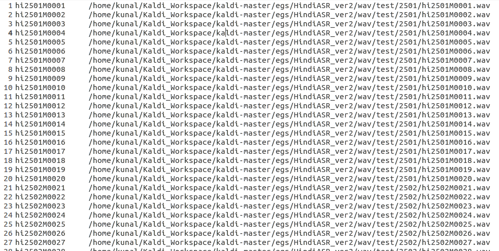
I followed the ID convention - first 2 letter signify Hindi , next four characters specify the speaker ID , the next character specifies the speaker gender(M or F) and the last four characters signify the sentence ID per speaker
Here , we would also normalize the extracted features with respect to the speaker to build a speaker independent model. For this we need to form two new files for both test and train data- 1) spk2utt and 2)utt2spk .
spk2utt gives us information about the sentences spoken by each speaker. For example, the spk2utt file for my test data is as follows:
Here the first entry is the speaker ID( we can notice that I have 7 speaker's data as I mentioned earlier) and that is followed by the sentence ID of each sentence spoken by that speaker
utt2spk gives us the information about who was the speaker for the given utterance(.wav file). For eg , the first few entries of the utt2spk file for my test data looks something like-
utt2spk gives us the information about who was the speaker for the given utterance(.wav file). For eg , the first few entries of the utt2spk file for my test data looks something like-
Next we create a file called text for both testing and training directories. This stores the word level transcription for each sentences (which are identified using their unique IDs as defined earlier). The first few entries for this file for my test data looks like:
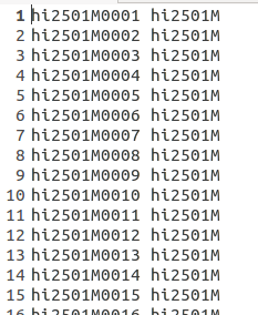
Last but not the least , we also create a file utt in both the test and train directories that list all the utterances ID present in that folder.
HINT: One need not manually prepare each of the above files. Assuming one has created the file wav.scp, the utt file can be created using the bash command
>cat wav.scp | awk '{print $1}' > utt
Now assuming only the first 7 characters correspond to the speaker info , rest signify the sentence info , we can create the file spk as follows:
>cat utt | cut -c 1-7 > spk
And the utterance to speaker file can now be easily created using :
>paste utt spk > utt2spk
and the corresponding spk2utt file can be generated with the help of a simple perl script present in the folder utils which is appropiately named as utt2spk_to_spk2utt.pl
Next we store the lexicon.txt that we had prepared for HTK earlier in the folder data/local/dict
In the same folder , we also create the following files :
Next , we start by creating the Language Model. We would be working with a N-gram Language model.
For my system , I choose the bi gram language model (can be changed by setting the value of variable n_gram to desired value in the script Create_ngram_LM.sh).
For this , we execute the command
> ./Create_ngram_LM.sh (ie we run the executable of the script Create_ngram_LM.sh)
Next , we have to build the acoustic model.
But before that we first check whether our folder structure is correct or not using the script fix_data_dir.sh present in the utils folder.
To do this , we run the command(from the parent directory):
> utils/fix_data_dir.sh data/train
> utils/fix_data_dir.sh data/test
Next we extract the features from the speech utterances. For this we run the command:
> steps/make_mfcc.sh - - nj 5 data/train exp/make_mfcc/train mfcc
Breaking down this command into parts to understand what this means:
We do the same thing for testing data
> steps/make_mfcc.sh - - nj 5 data/test exp/make_mfcc/test mfcc
Next we perform the speaker normalization. For thus we run the bellow commands:
> steps/compute_cmn_stats.sh data/train exp/make_mfcc/train mfcc
> steps/compute_cmn_stats.sh data/test exp/make_mfcc/test mfcc
Then we again validate whether the data is present appropriately as required for modelling. To do this , we run the commands:
>utils/validate_data_dir.sh data/train
>utils/validate_data_dir.sh data/test
Now we train the monophone system. Again here we use the flat start approach ( ie when the phone boundaries are not given as in our case, we divide frames equally among all phones to start ). The command for this is
>steps/train_mono.sh - - nj 10 data/train data/lang_bigram exp/mono
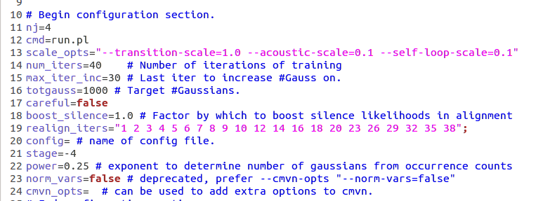
As I had stated earlier, the algo doesnt try to fit the same number of gaussians for each phone , rather it iteratively looks for the best number of gaussians for each state. We just specify the total number of gaussians we want (which serves the max limit) in the config file. Please find below a small part of the config file where we specify the total number of Gaussians required:
HINT: One need not manually prepare each of the above files. Assuming one has created the file wav.scp, the utt file can be created using the bash command
>cat wav.scp | awk '{print $1}' > utt
Now assuming only the first 7 characters correspond to the speaker info , rest signify the sentence info , we can create the file spk as follows:
>cat utt | cut -c 1-7 > spk
And the utterance to speaker file can now be easily created using :
>paste utt spk > utt2spk
and the corresponding spk2utt file can be generated with the help of a simple perl script present in the folder utils which is appropiately named as utt2spk_to_spk2utt.pl
Next we store the lexicon.txt that we had prepared for HTK earlier in the folder data/local/dict
In the same folder , we also create the following files :
- non_silence_phones.txt : this contains all the phones present in the lexicon
- optional_silence.txt: for our scenario , this only contains the silence sil
- silence_phones.txt : contains the sounds that do not contain acoustic information, but are present like noises(also called fillers)
Next , we start by creating the Language Model. We would be working with a N-gram Language model.
For my system , I choose the bi gram language model (can be changed by setting the value of variable n_gram to desired value in the script Create_ngram_LM.sh).
For this , we execute the command
> ./Create_ngram_LM.sh (ie we run the executable of the script Create_ngram_LM.sh)
Next , we have to build the acoustic model.
But before that we first check whether our folder structure is correct or not using the script fix_data_dir.sh present in the utils folder.
To do this , we run the command(from the parent directory):
> utils/fix_data_dir.sh data/train
> utils/fix_data_dir.sh data/test
Next we extract the features from the speech utterances. For this we run the command:
> steps/make_mfcc.sh - - nj 5 data/train exp/make_mfcc/train mfcc
Breaking down this command into parts to understand what this means:
- steps/make_mfcc.sh : this is the script file that would compute the MFCC coefficients
- - - nj 5: this means break the above work to 5 number of jobs
- data/train: location of the training data
- exp/make_mfcc/train: location to store the log files
- mfcc : name of the folder where the extracted feature files would be stored
We do the same thing for testing data
> steps/make_mfcc.sh - - nj 5 data/test exp/make_mfcc/test mfcc
Next we perform the speaker normalization. For thus we run the bellow commands:
> steps/compute_cmn_stats.sh data/train exp/make_mfcc/train mfcc
> steps/compute_cmn_stats.sh data/test exp/make_mfcc/test mfcc
Then we again validate whether the data is present appropriately as required for modelling. To do this , we run the commands:
>utils/validate_data_dir.sh data/train
>utils/validate_data_dir.sh data/test
Now we train the monophone system. Again here we use the flat start approach ( ie when the phone boundaries are not given as in our case, we divide frames equally among all phones to start ). The command for this is
>steps/train_mono.sh - - nj 10 data/train data/lang_bigram exp/mono
As I had stated earlier, the algo doesnt try to fit the same number of gaussians for each phone , rather it iteratively looks for the best number of gaussians for each state. We just specify the total number of gaussians we want (which serves the max limit) in the config file. Please find below a small part of the config file where we specify the total number of Gaussians required:
Hint: After the above training of monophone system is complete, we can check the total number of gaussians assigned to each state and other parameters using the command:
> gmm-info exp/mono/final.mdl
Next we form the graph for our model. This is done via the command
> utils/mkgraph.sh - - mono data/lang_bigram exp/mono exp/mono/graph
This combines the acoustic and language model information and best symbolises our trained system.
Now comes the Decode step. Here we check how our system performs to unseen testing data . The command for the same is :
steps/decode.sh - -nj 5 exp/mono/graph data/test exp/mono/decode
here we evaluate our model for different LM weights ( the output depends on language model and acoustic model, we have to decide what confidence score we want to give to prediction of both the models, because the final output will be prediction of each model multiplied by their weights) . We do this so as to tune this hyper-parameter and we finally select the the weight that gives minimum error. Thus we take the result as the one corresponding to the weight that gives minimum WER(word error rate). The output for our model is:
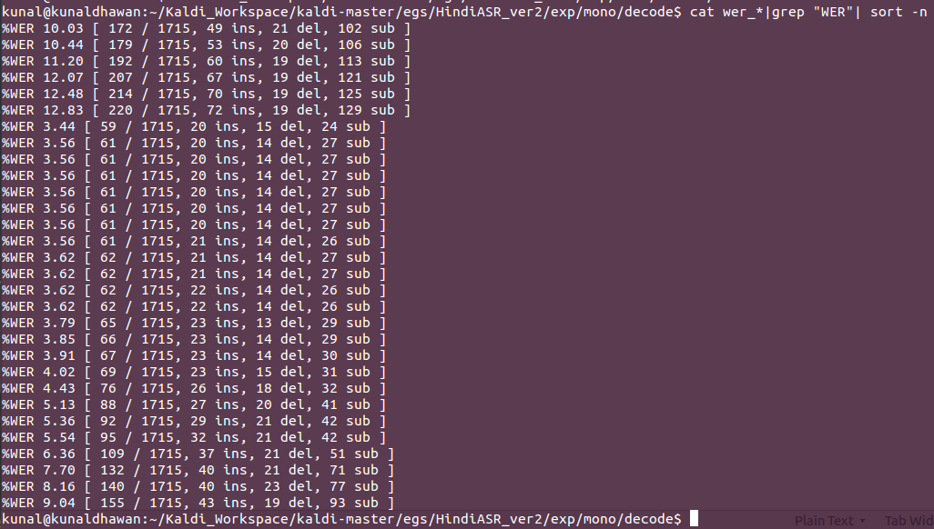
Thus our monophone-HMM has a best performance in which the word error rate is just 3.44% , where only 59 out of 1715 were decoded incorrectly from the testing data. We can clearly observe the difference between HTK and Kaldi model where the only difference was different number of gaussians for each model and adjustable language model and acoustic weights.
Next I try to build a triphone-HMM system
Next I try to build a triphone-HMM system
2) Triphone HMM System
A triphone is a sequence of three phonemes.Triphones are useful in models of natural language processing where they are used to establish the various contexts in which a phoneme can occur in a particular language.
Basically here we try to model all possible combinations 3 consecutive phonemes present in training data using one HMM model and then try to decode the testing information using these models only. This helps us because triphones bring with them contextual information , ie the knowledge that this given phoneme can occur with which other phonemes. This helps us make better/more informed choices while decoding because we know that which phoneme out of our given dictionary is more probable to occur after the previous identified phone. This may not help in limited vocabulary problems (eg number recognition problem) where the phone/word order plays no significance , but in the case of recognition of continuous meaningful sentences , it performs better than monophone systems
Here I would proceed to show how to build the triphone system from previously built monophone system.
Firs we align the monophone system to get the phone boundaries. Also we boost silence so that our system works better in noisy environment. As per the code below, energy=silence energy*1.25 is also taken as silence only. The command to be executed is :
> steps/align_si.sh - - boost-silence 1.25 - - nj 5 data/train data/lang_bigram exp/mono exp/mono_ali
Next we train the triphone model
> steps/train_deltas.sh 2000 16000 delta/train data/lang_bigram exp/mono_ali exp_tri
here the 2000 is the parametric value of the max number of senons we want to fit and 16000 the parametric value of the maximum number of gaussians to modelled (both these values depend data thus different values should be tried and the best one should be used)
Now , as we did in monophone system , we make the graph by running
> utils/mkgrapgh.sh data/lang_bigram exp/tri exp/tri/graph
And then we decode
>steps/decode.sh - - nj 5 exp/tri/graph data/test exp/tri/decode
Again this gives us files for different LM weight that we have set in the config file. Sorting the different results , we obtain :
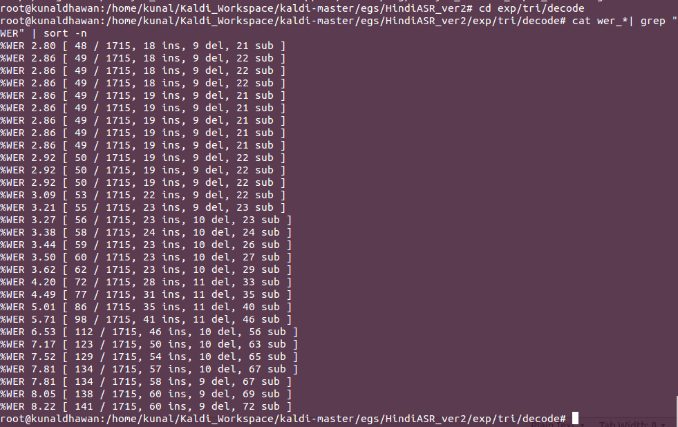
Thus we best get a model which has a word error rate of only 2.80 %
3)DNN-HMM System
Here we model the sates of the hidden Markov model as a Deep Neural Network instead of modelling it via a Gaussian mixture model. Thus the state transition probabilities remain the same as the above triphone model , just that now the state observing/emission probability will be modelled by a Deep Neural Network.
Best resource for learning about the basics and theory of DNN would be the course 1 of the deeplearning.ai specialization on Coursera. I too referred the same for the theory www.coursera.org/account/accomplishments/certificate/VTWWCBH3AE6W . Another important reference for the same is Hinton Sir's paper Deep Neural Networks for Acoustic Modeling in Speech Recognition ( link - ieeexplore.ieee.org/document/6296526/ )
Again, first we align the previous triphone model via the code
> steps/align_si.sh - - nj 5 data/train data/lang_bigram exp/tri exp/tri_ali
Now reusing the state transition model and training the DNN state emission model , we run the following command:
> steps/nnet2/train_tanh.sh - -initial-learning-rate 0.015 - -final-learning-rate 0.002 - -num-hidden-layers 1 - -minibatch-size 128 - -hidden-layer-dim 256 - -num-jobs-nnet 10 - -num-epochs 5 data/train data/lang_bigram exp/tri_ali exp/DNN
explaining this command-
After this we check for the working of our model on test data by running the decode command:
> steps/nnet2/decode.sh --nj 4 exp/tri/graph data/test exp/DNN/decode
Finally checking for the best weight for language model , we obtain the result as:
Here we model the sates of the hidden Markov model as a Deep Neural Network instead of modelling it via a Gaussian mixture model. Thus the state transition probabilities remain the same as the above triphone model , just that now the state observing/emission probability will be modelled by a Deep Neural Network.
Best resource for learning about the basics and theory of DNN would be the course 1 of the deeplearning.ai specialization on Coursera. I too referred the same for the theory www.coursera.org/account/accomplishments/certificate/VTWWCBH3AE6W . Another important reference for the same is Hinton Sir's paper Deep Neural Networks for Acoustic Modeling in Speech Recognition ( link - ieeexplore.ieee.org/document/6296526/ )
Again, first we align the previous triphone model via the code
> steps/align_si.sh - - nj 5 data/train data/lang_bigram exp/tri exp/tri_ali
Now reusing the state transition model and training the DNN state emission model , we run the following command:
> steps/nnet2/train_tanh.sh - -initial-learning-rate 0.015 - -final-learning-rate 0.002 - -num-hidden-layers 1 - -minibatch-size 128 - -hidden-layer-dim 256 - -num-jobs-nnet 10 - -num-epochs 5 data/train data/lang_bigram exp/tri_ali exp/DNN
explaining this command-
- steps/nnet2/train_tanh.sh : we use the tanh activation function
- - -initial-learning-rate 0.015 - -final-learning-rate 0.002 : for the initial estimation we use the learning rate alpha as 0/015 and towards convergence we reduce it to 0.002
- - -num-hidden-layers 1: I use only 1 hidden layer( though more number of hidden layers would lead to better performance , but due to very less data and less computational resources , I preferred to use only 1 hidden layer
- - -minibatch-size 128: size of mini batch is 128
- - -hidden-layer-dim 256: dimension of the hidden layer = 256
- - -num-jobs-nnet 10 : number of jobs =10
- - -num-epochs 5: number of epochs =5
- data/train: location of training data
- data/lang_bigram : location of language model
- exp/tri_ali: location of aligned triphone models
- exp/DNN: where to store the new models
After this we check for the working of our model on test data by running the decode command:
> steps/nnet2/decode.sh --nj 4 exp/tri/graph data/test exp/DNN/decode
Finally checking for the best weight for language model , we obtain the result as:
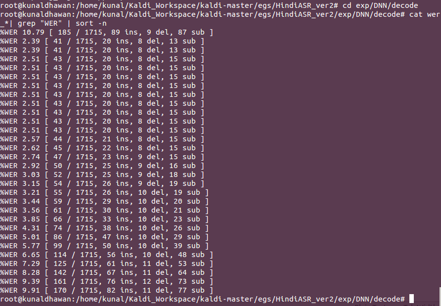
Thus our best system gave a Word error rate of 2.39 %. This is remarkably good given the fact that I used only 1 hidden layer , hidden layer dimension of 256 , number of epochs as 5 only. Given more data and thus more hidden layers and number of epochs , this result will only improve (if it doesnt leads to over-fitting which can be taken care by regularization)
This marks the end of the documentation. I really enjoyed working on this project and this was a steep learning curve. But this is just the beginning and I would try to work on more complex research projects in the next few months.
This marks the end of the documentation. I really enjoyed working on this project and this was a steep learning curve. But this is just the beginning and I would try to work on more complex research projects in the next few months.
